Comparison of Volatility Estimators
Posted on Sun 07 March 2021 in Volatility
Today, I'm going to be discussing the difference between two volatility estimators.
The Data
I'm going to be using daily-resolution SPX data from Sharadar as well as minute-resolution SPX data from First Rate Data.
import pandas as pd
import numpy as np
import sqlite3
from matplotlib import pyplot as plt
from scipy import stats

# Set default figure size
plt.rcParams["figure.figsize"] = (15, 10)
conn = sqlite3.Connection("data.db")

spx_daily = pd.read_sql("SELECT * FROM prices WHERE ticker='^GSPC'", conn, index_col="date", parse_dates=["date"])
spx_minute = minute = pd.read_csv("SPX_1min.csv", header=0,names=['datetime', 'open', 'high', 'low', 'close'],
                                  index_col='datetime', parse_dates=True)
# A quick look at the data
spx_daily.head()
| ticker | open | high | low | close | volume | dividends | closeunadj | lastupdated | |
|---|---|---|---|---|---|---|---|---|---|
| date | |||||||||
| 1997-12-31 | ^GSPC | 970.84 | 975.02 | 967.41 | 970.43 | 467280000 | 0 | 970.43 | 2019-02-03 |
| 1998-01-02 | ^GSPC | 970.43 | 975.04 | 965.73 | 975.04 | 366730000 | 0 | 975.04 | 2019-02-03 |
| 1998-01-05 | ^GSPC | 975.04 | 982.63 | 969.00 | 977.07 | 628070000 | 0 | 977.07 | 2019-02-03 |
| 1998-01-06 | ^GSPC | 977.07 | 977.07 | 962.68 | 966.58 | 618360000 | 0 | 966.58 | 2019-02-03 |
| 1998-01-07 | ^GSPC | 966.58 | 966.58 | 952.67 | 964.00 | 667390000 | 0 | 964.00 | 2019-02-03 |
spx_minute.head()
| open | high | low | close | |
|---|---|---|---|---|
| datetime | ||||
| 2007-04-27 12:25:00 | 1492.39 | 1492.54 | 1492.39 | 1492.54 |
| 2007-04-27 12:26:00 | 1492.57 | 1492.57 | 1492.52 | 1492.56 |
| 2007-04-27 12:27:00 | 1492.58 | 1492.64 | 1492.58 | 1492.63 |
| 2007-04-27 12:28:00 | 1492.63 | 1492.73 | 1492.63 | 1492.73 |
| 2007-04-27 12:29:00 | 1492.91 | 1492.91 | 1492.87 | 1492.87 |
The Estimators
Now, what I want to do is compare volatility estimates from these two data sets. I would prefer to use the daily data if possible, because in my case it's easier to get and updates more frequently.
Garman-Klass Estimator
This estimator has been around for a while and is deemed to be far more effcient than a traditional close-to-close volatility estimator (Garman and Klass, 1980).
From equation 20 in the paper, a jump adjusted volatility estimator:
\(f = 0.73\), percentage of the day trading is closed based on NYSE hours of 9:30 to 4
\(a = 0.12\), as they suggest in the paper
\(\sigma^2_{unadj} = 0.511(u - d)^2 - 0.019(c(u+d) - 2ud) - 0.383c^2\)
\(\sigma^2_{adj} = 0.12\frac{(O_{1} - C_{0})^2}{0.73} + 0.12\frac{\sigma^2_{unadj}}{0.27}\)
Where,
\(u = H_{1} - O_{1}\), the normalized high
\(d = L_{1} - O_{1}\), the normalized low
\(c = C_{1} - O_{1}\), the normalized close
and subscripts indicating time. They also indicate in the paper that these equations expect the log of the price series.
def gk_vol_calc(data):
    u = np.log(data['high']) - np.log(data['open'])
    d = np.log(data['low']) - np.log(data['open'])
    c = np.log(data['close']) - np.log(data['open'])
    vol_unadj = 0.511 * (u - d)**2 - 0.019 * (c * (u + d) - 2 * u * d) - 0.283 * c**2

    jumps = np.log(data['open']) - np.log(data['close'].shift(1))
    vol_adj = 0.12 * (jumps**2 / 0.73) + 0.12 * (vol_unadj / 0.27)

    return vol_adj
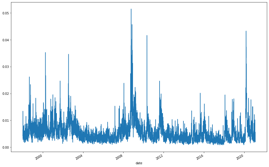
# Let's take a look
gk_vol = np.sqrt(gk_vol_calc(spx_daily))
gk_vol.plot()
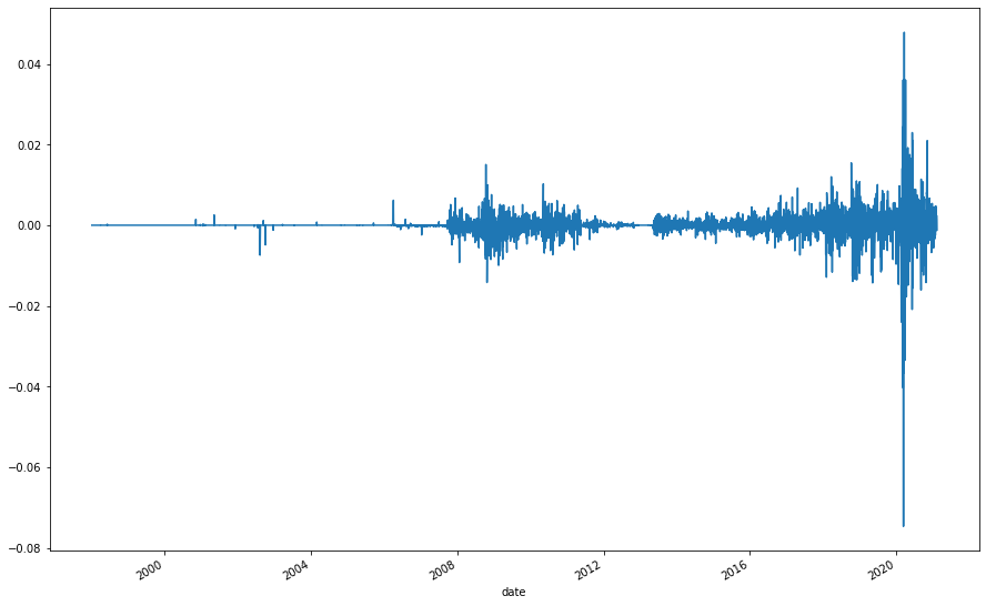
As an aside, opening jumps have become more common and larger in recent years, maybe something to investigate. This is as a percentage, so it's not a simple case of the index values becoming larger.
(spx_daily['open'] / spx_daily['close'].shift(1) - 1).plot()
Realized Volatility Estimator
This estimator is very simply and has become more prominent in the literature in the last few years because of increasing availability of higher-frequency data. Based on (Liu, Patton, and Sheppard, 2012), it's hard to beat a 5-minute RV. Here, I'm going to use a 1-minute estimator, which is also shown to be effective.
\(RV_{t} = \sum_{k=1}^n r_{t,k}^2\), where the \(t\) index is each day, and the \(k\) index represents each intraday return
For daily volatility, it's simply a sum of squared returns from within that day. So in this case we calculate returns for each 1 minute period, square them, and they sum them for each day.
def rv_calc(data):
    results = {}

    for idx, data in data.groupby(data.index.date):
        returns = np.log(data['close']) - np.log(data['close'].shift(1))
        results[idx] = np.sum(returns**2)

    return pd.Series(results)
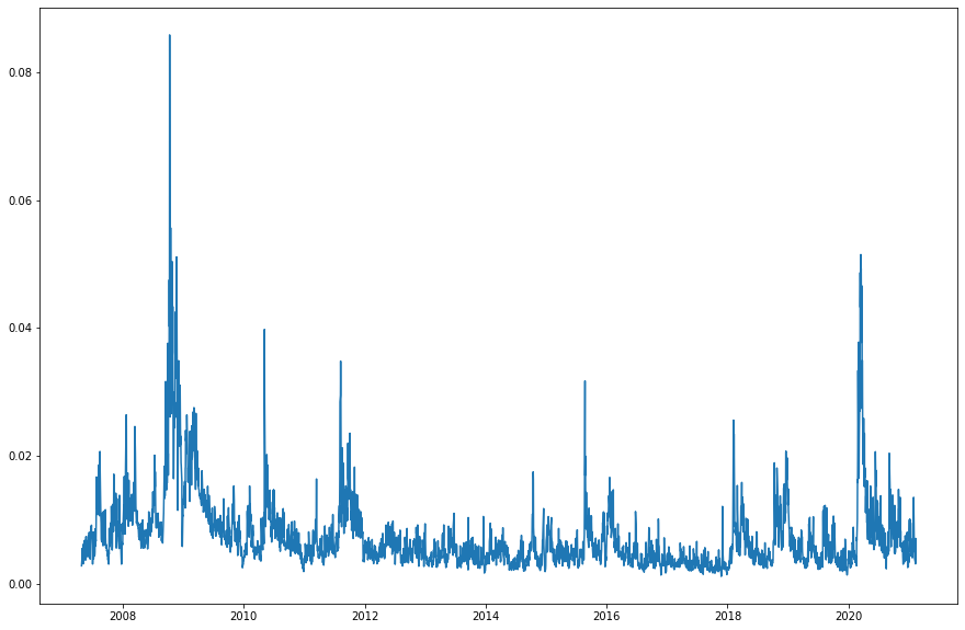
# Let's take a look at this one
rv = np.sqrt(rv_calc(spx_minute))
rv.plot()
Comparisons
# Because the minute data has a shorter history, let's match them up
gk_vol = gk_vol.reindex(rv.index)
rv.plot()
gk_vol.plot()
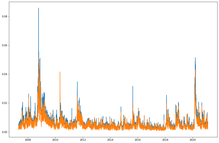
Here's a plot of our two different volatility estimators with RV in blue and Garman-Klass in orange. The RV estimator is far less noisy, looking at each of their graphs above. The Garman-Klass estimator also seems to persistently return a lower result than RV. This is backed up by looking at a graph of their difference.
(gk_vol - rv).plot()
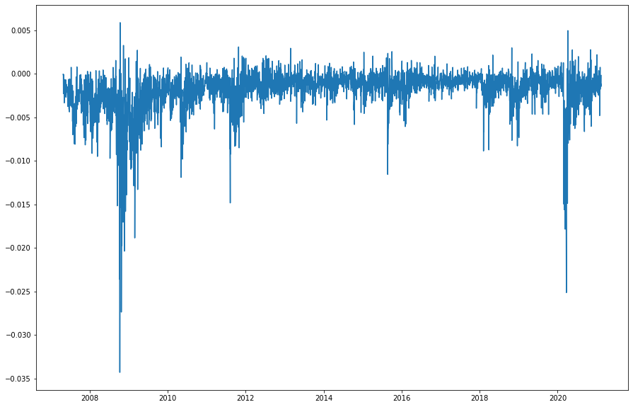
Netx, let's analyze how they do at normalizing the returns of the S&P 500. According to (Molnár, 2015) normalizing a number of equity returns by their Garman-Klass estimated volatility does indeed make their distributions normal. Let's see if we can replicate that result with either of our esimates on the S&P 500.
# Daily close-to-close returns of the S&P 500
spx_returns = np.log(spx_daily['close']) - np.log(spx_daily['close'].shift(1))
spx_returns = spx_returns.reindex(rv.index)
# Normalizing by our estimated volatilties
gk_vol_norm = (spx_returns / gk_vol).dropna()
rv_norm = (spx_returns / rv).dropna()
# Here are the unadjusted returns
_, _, _ = plt.hist(spx_returns, bins=50)

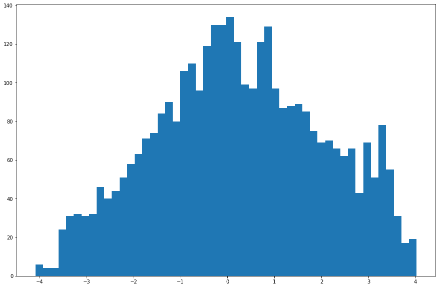
# Here's normalized by the Garman-Klass Estimator
_, _, _ = plt.hist(gk_vol_norm, bins=50)
# And this is by the RV estimator
_, _, _ = plt.hist(rv_norm, bins=50)
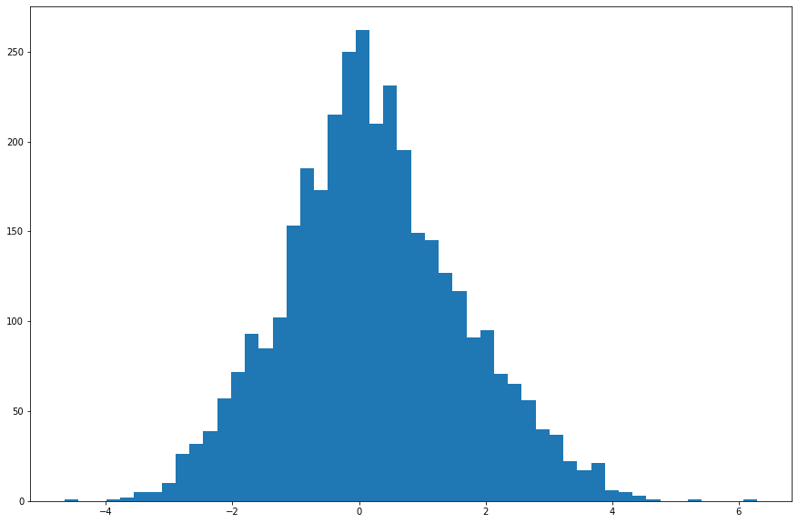
At first glance, the RV adjusted returns seem most like normal to me, let's run some tests. These Scipy tests set the null hypothesis that the data comes from a corresponding normal distribution. So if the p-value is small we can reject that hypothesis and conclude the distribution is non-normal.
print(stats.skewtest(gk_vol_norm))
print(stats.skewtest(rv_norm))
    Garman-Klass Skew: SkewtestResult(statistic=-0.3767923327324783, pvalue=0.7063279391177064)
    RV-5min Skew: SkewtestResult(statistic=5.251294175425576, pvalue=1.5103423951480544e-07)
print(stats.kurtosistest(gk_vol_norm))
print(stats.kurtosistest(rv_norm))
    KurtosistestResult(statistic=-13.088609427904334, pvalue=3.825472809774632e-39)
    KurtosistestResult(statistic=0.315320709120601, pvalue=0.7525181628202805)
Looks like the Garman-Klass-normalized returns have normal skew, but non-normal kurtosis. The RV-normalized returns have non-normal skew but normal kurtosis! There's no winning here! Both are non-normal in different ways. Either normalization does do better than the unadjusted returns though.
print(stats.skewtest(spx_returns.dropna()))
print(stats.kurtosistest(spx_returns.dropna()))
    SkewtestResult(statistic=-12.386230904806132, pvalue=3.1028724633560147e-35)
    KurtosistestResult(statistic=26.470418979318143, pvalue=2.124045513612033e-154)
Conclusion
While from a statistical point of view, neither option seems particularly favorable, my personal choice is going to be the RV estimator. I think the literature is clear on its efficacy and its less noisy and conceptually easier. It's been said that when there are a bunch of competing theories, none of them are very good. So I'll pick the simplest option and go with RV.
References
-
Garman, M., & Klass, M. (1980). On the Estimation of Security Price Volatilities from Historical Data. The Journal of Business, 53(1), 67-78. Retrieved February 14, 2021, from http://www.jstor.org/stable/2352358
-
Liu, L., Patton, A., & Sheppard, K. (2012). Does Anything Beat 5-Minute RV? A Comparison of Realized Measures Across Multiple Asset Classes. SSRN. http://dx.doi.org/10.2139/ssrn.2214997
-
Molnár, P. (2015). Properties of Range-Based Volatility Estimators. SSRN. Retrieved from https://ssrn.com/abstract=2691435